This is a new entry on the broad theme of electrophysiological Biomarkers and Predicting pathological states disease from resting state EEG analysis.
I am interested in excitatory to inhibitory (E/I) balance quantification from electrophysiological data, especially in non invasive recordings where the direct evaluation of this balance is not possible (e.g. EEG data). Excitation and inhibition disbalance are cardinal phenomena in neural pathology (e.g. epilepsy, Alzheimer’s) and can be directly assessed via advanced in vitro neurophysiological methods from neurosurgical tissue but the quantification of such a balance from EEG has been challenging. Recent attempts on evaluating excitation inhibition balance (E/I) have focused on some previously unsuspected entity. The Aperiodic elements of the power spectrum.
Spectral Analysis of electrophysiological signals transform a time series into a Power Frequency times series allowing for the decomposition and separation of oscillatory and non oscillatory parts/patterns in the signal. Even though the oscillatory patterns and oscillatory behavior in the brain has been well characterized, the more subtle ,albeit, background and omnipresent elements of the spectral decomposition (collectively know as the aperiodic element of the spectrum) are generally overlooked by most research groups.
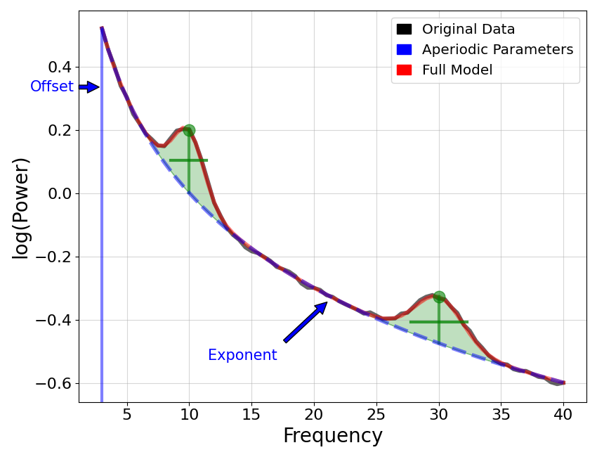
It all started with a series of manuscripts (Gao et al., 2017 Neuroimage) asking the question. ‘Does the 1/f (one over frequency) power law of the non oscillatory elements of the EEG (i.e. the aperiodic signal) encode something meaningful for the brain ? But what is 1/f one might asks (see opening image taken from https://fooof-tools.github.io/fooof/). By ‘aperiodic’ activity or 1/f or 1/f scaling, we mean activity that is not rhythmic, or activity that has no characteristic frequency. In the power spectrum, this is seen as 1/f-like activity, whereby (in linear space) the power across frequencies decreases with a relationship 1/f **x. The x we call the exponent of the aperiodic element of the power spectrum.
To measure the aperiodic activity, we would like to describe the pattern of activity across all frequencies, without our measure being influenced by co-occurring periodic activity (peaks). Gao and colleagues have created a special python library to help dissect out the periodic and aperiodic elements of the neural spectral analysis called FOOOF (https://fooof-tools.github.io/fooof/index.html). They then went on to show that the aperiodic exponent described the E/I balance in both computational models of networks of inhibitory and excitatory cells but also in behavioral anesthesia.
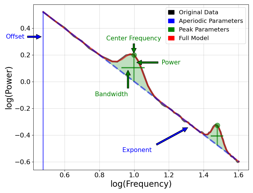
Mathematical Description of the Aperiodic Spectral Component:
To fit the aperiodic component of the power spectrum of the neural signal, Gao used the function L:
where L(F) = b- log(k + F**x). Note that this function is fit on the semi-log power spectrum, meaning linear frequencies and power values.
In this formulation, the parameters b, k and x, , and define the aperiodic component, as: b is the broadband ‘offset’; k is the ‘knee’ of the spectrum ; x is the ‘exponent’ of the aperiodic fit; F is the array of frequency values
Experimental determination of E/I balance in a computational model
To simplify the matter and to follow the results of Gao et al., 2017, I have asked the following question. How does 1/f (aperiodic 1/f exponent and linear slope determination) change in a single compartment neuron bombarded by random excitation and varying strength of random inhibition? In other words how does the excitation inhibition balance looks at the cellular level in the most simple of cases.
In order to make the models as stripped down as possible, I have used a published substantia Nigra par compacta neuron model that I have constructed in the past (NEURON simulation environment, Ortner et al., 2017 J Neurosci, https://modeldb.science/2017402 ) and added synaptic mechanisms of AMPA and GABA receptors as a two exponential synapse (typical rise tau and decay tau). Synapses are activated by a NEURON NetCon object at random times centered around a mean activation interval (set at 20 ms, i.e. 50 Hz for both types of synapses). Simulations were run for 10 seconds at 50 KHz.
model_parameters =
{‘AMPA_activation_interval’: 20, ‘GABA_activation_interval’: 20, ‘rev_syn_AMPA’ : 0, ‘rev_syn_GABA’ : -80, ‘tau_rise_AMPA’ : 0.3,’tau_decay_AMPA’ : 2, ‘tau_rise_GABA’ : 0.5,’tau_decay_GABA’ : 10, ‘AMPA_G’ : 0.0002, ‘GABA_G’: VARIABLE }
I have systematically varied the neuron’s inhibitory conductance (in 12 steps) while keeping the AMPAergic drive constant to achieve E/I balances of 1 over [ 0.25, 0.5, 1, 1.5, 2.0, 2.5, 3.0, 3.5, 4.0, 4.5, 5.0, 5.5, 6.0 ]. I have run 5 replicates of every simulation at each E/I balance for statistical inferences.
I have calculated the extracellular voltage from the somatic voltage trajectory at a distance of 200 micrometers (with extracellular conductivity at typical 0.3 S/m) from the soma using the summation of the transmembrane currents (a manual implementation of the Ness and colleagues method 2022 Exp Med Biol)
i_memb = (i_cap + i_AMPA + i_GABA + i_NaF * nA_Factor + i_kD * nA_Factor + i_leak * nA_Factor + i_kA * nA_Factor + i_H * nA_Factor + i_kM * nA_Factor + i_CaW * nA_Factor + i_NaP * nA_Factor + i_kCa * nA_Factor + i_capump * nA_Factor)
where nA factor is the conversion factor of the ionic densities to current (nA). Note the neuron operates with ten (10) different conductances including a fast (NaF) and a persistent (NaP) sodium channel, a leak current (leak), combined calcium currents (CaW), a hyperpolarisation activated cation current (H-current), an extruding calcium pump (capump), four potassium currents (a Delayed rectifier type current, an M- type current, a kCa calcium activated potassium current and an A-type current)
Finally, I run two variants of the model, one where the soma has entirely passive properties and one that has all active properties activated (referred herein as active and passive models).
The first two figures attached (the title of figure details the model used, ACTIVE or PASSIVE model). Below is a simple explanation on what you see herein
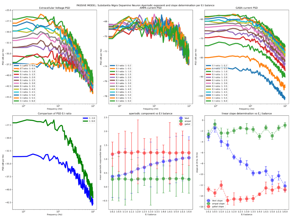
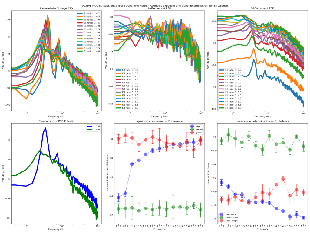
The first row shows the Welch PSD of the extracellular voltage (left panel) as well as the PSD of the AMPA (middle panel) and GABA (right panel) current densities (from left to right). The second row (left panel) shows a comparative example of two representative extracellular voltage PSDs (depicting 1:2 and 1:6 E/I balances, chosen to reflect the choices of Gao et al., 2017 Neuroimage). The fitted aperiodic component to the PSD (using the FOOOF library) is depicted in the middle panel and the linear slope determination (fit chosen in range 20 to 70 Hz, it does not change the qualitative results if flexed around> 20 <100 Hz) is shown on the right panel.
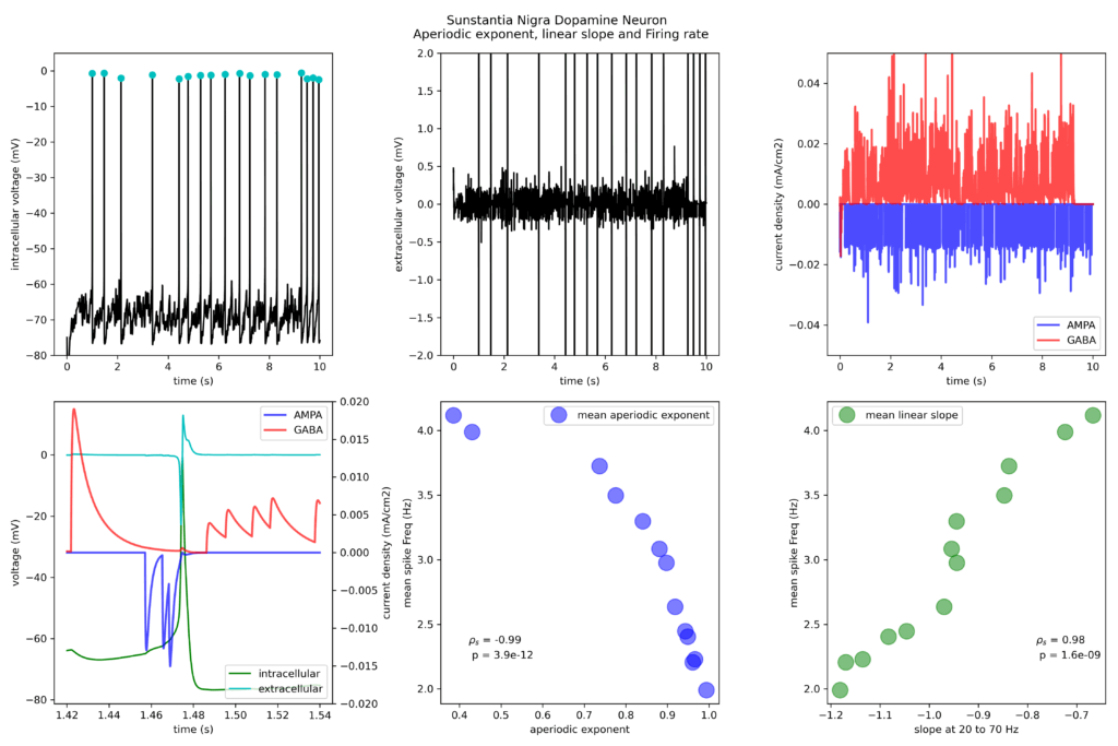
Finally, to follow up the results I have also correlated the firing rate with the extracted aperiodic exponent and linear slope on the active model. On the first row, I depict typical action potential firing of the model neuron (intracellular potentials and calculated extracellular potentials 200 micm away from the neuron, left and middle panel respectively) that arise from the stochastic train of AMPA and GABA activations (right panel). On the bottom row, I show an example of overlay of traces of the aforementioned experimental design (left panel) followed by the correlation (Spearman’s correlation rho and probability) of firing rate against aperiodic exponential (middle panel) and linear slope (right panel).
Conclusions: Can the E/I balance predicted via aperiodic spectral analysis?
Based on the systematic experimental approach introduced above, the following observations have been made:
Increasing the inhibitory drive in either the active or passive model results in a larger aperiodic exponent (bottom row, middle panel), while the linear slope determined becomes steeper (evident by the more negative slope) with increased strength of the inhibitory drive (bottom row, right panel). The firing rate of the neuron strongly and significantly correlated with both aperiodic (negatively) and linear slope (positively) pointing out that the inhibitory conductance sets a tone for neuron output as expected.
These results suggest that in a minimalistic single compartment model, inhibitory drive (and by extension E/I balance) is reflected on both the fitted aperiodic exponent and the slope determinants. These results seem to confirm the model of Gao and colleagues where more inhibition results in steeper PSD linear slopes. Is this the whole story then? By far no. In the next blog I will explore E)I balance and aperiodic parameters in a morphologically complex model of human cortical neuron.